What happens when you combine a data nerd with a self-described movie buff? Far too much nonsense.
For the last few years, I have been recording my daily activities and moods using a nifty app called Daylio. I wanted a way to record what I did day to day in a less formalized way than journaling. Along with my general daily routine, I recorded every time I watched a movie as well as my personal rating (out of 10) of the movie. I decided to create a spreadsheet of all of the movies that I watched in 2020 based on all of those entries.
I’ll start with the statistical and graphical analyses of the data that I generated. I am including my R code – if that doesn’t interest you, just look at the pretty graphs. If you are only interested in my movie awards for the year, feel free to scroll towards the bottom of the page.
The Data

Here’s the top of the dataset. The release year, directors, MPA rating and medium were all directly taken from IMDB. Genres tend to be all over the place on IMDB, so I restricted the possibilities to what I considered the movie’s “main” genre, and added a secondary genre if I felt it needed nuance. I included a column to denote if I had previously watched the movie. Lastly, I recorded my personal rating of the movie.
There’s nothing that I love more than a fresh dataset (go ahead, call me a nerd, I DARE you). Using R, I began to play around with the dataset I had created.
The quick facts upfront: In the last year, I watched 75 films (as of 12/27/2020). The vast majority of those were from the 2010s. 19 of those 75 movies were re-watches.
## Packages used
library(ggplot2)
library(doBy)
library(dplyr)
## Import file
m = read.csv("C:/filepath/moviesmaster.csv")
dim(m)
[1] 75 23
Cleaning the dataset:
## Selecting just the rows that I'm interested in for the analysis
column = c("title","year","director1","genre1","genre2","personal_rating", "rewatch", "watchdate", "mpa")
m = m[,column]
## Changing the vairables to the correct class type
nums = c("personal_rating","year")
nonnums = c("genre1","genre2","rewatch","mpa")
m[nums] = sapply(m[nums],as.numeric)
m[nonnums] = sapply(m[nonnums],as.character)
## There are a few NAs that I don't want to mess up the analysis
m = na.omit(m)
## Making a decades column
m$decade = m$year - m$year %% 10
Plotting movies watched by decade:
## Creating a table
dec = as.data.frame(table(m$decade))
names(dec)[1] = "dec"
names(dec)[2] = "freq"
## Plotting table with ggplot
gdec = ggplot(data = dec, aes(x = dec, y = freq, fill=dec))
gdec + geom_col() + labs(title="Movies watched in 2020 by decade", x = "Decade", y = "Total number")
+ theme(text = element_text(size=15), legend.position = "none")
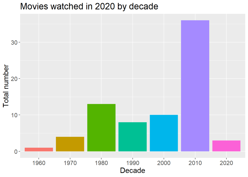
This year, some friends and I started a horror movie club, where we voted on a horror movie to watch each week. Because of this, horror dominated this year.
## Finding the number of movies by genre1
gen = as.data.frame(table(m$genre1))
names(gen)[1] = "genre"
names(gen)[2] = "freq"
## Reordering it from largest to smallest
gen = transform(gen, genre = reorder(genre, -freq))
## Plotting with ggplot
ggen = ggplot(data = gen, aes(x=genre, y=freq, fill = genre))
ggen + geom_col() + labs(title="Movies watched in 2020 by primary genre", x = "Genre", y = "Total number") +
  theme(text = element_text(size=15), axis.text.x = element_text(angle = 90), legend.position = "none")
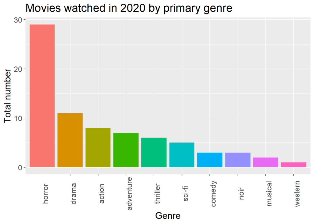
Quick note on genre – as I said before, this is just based on how I primarily see the movie. If I was conflicted or wasn’t completely sure what to choose, I would default to IMDB’s classifications.
Considering I watched so much horror this year, I find it unsurprising that so many of the movies I watched were rated R.
rat = as.data.frame(table(m$mpa))
names(rat)[1] = "mpa"
names(rat)[2] = "freq"
## plotting with ggplot
rat = transform(rat, mpa = reorder(mpa, -freq))
grat = ggplot(data = rat, aes(x=mpa, y=freq, fill = mpa))
grat + geom_col() + labs(title="Movies watched in 2020 by MPA Rating", x = "Rating", y = "Total number") +
  theme(text = element_text(size=15), axis.text.x = element_text(angle = 0), legend.position = "none")

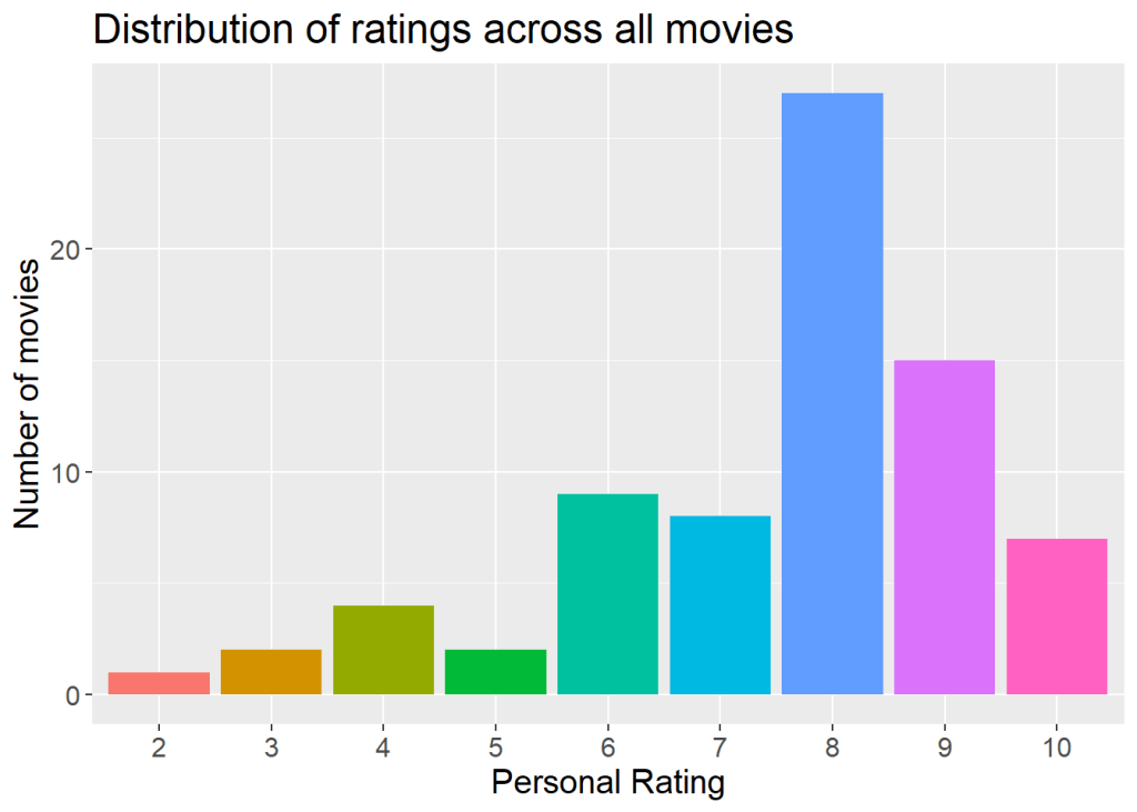
Below is a plot of the distribution of ratings that I gave over the year. Seems like it was a pretty good year overall, with most movies being rated around an 8. I didn’t technically have any 10s this year, but since I rounded to the nearest whole number for this plot, 9.5s and higher were rounded to 10.
## Creating a column of rounded ratings
m$roundrating = round(m$personal_rating, 0)
## Creating a table of the ratings
rat_dist = as.data.frame(table(m$roundrating))
names(rat_dist)[1] = "rating"
names(rat_dist)[2] = "freq"
## Plotting table with ggplot
grat_dist = ggplot(data = rat_dist, aes(x =rating, y = freq, fill=rating))
grat_dist + geom_col() +
labs(title="Distribution of ratings across all movies", x = "Personal Rating", y = "Number of movies") +
theme(text = element_text(size=15), legend.position = "none")
I had hypothesized that older movies would likely be rated disproportionately higher, due to what I’m now dubbing “the Classics Effect”. If I watch a movie from the 70’s, it’s likely because the movie is still worth watching, thus potentially creating a bias of higher ratings for older movies.
avgdec = summaryBy(personal_rating~decade, data = m, FUN = mean, na.rm = TRUE)
names(avgdec)[1] = "decade"
names(avgdec)[2] = "avg_rating"
gavgdec = ggplot(data = avgdec, aes(x=decade, y=avg_rating, fill = decade))
gavgdec + geom_col() +
labs(title="Average rating by decade", y = "Average Personal Rating (1-10)", x="Decade of movie release") + theme(text = element_text(size=15), legend.position = "none")
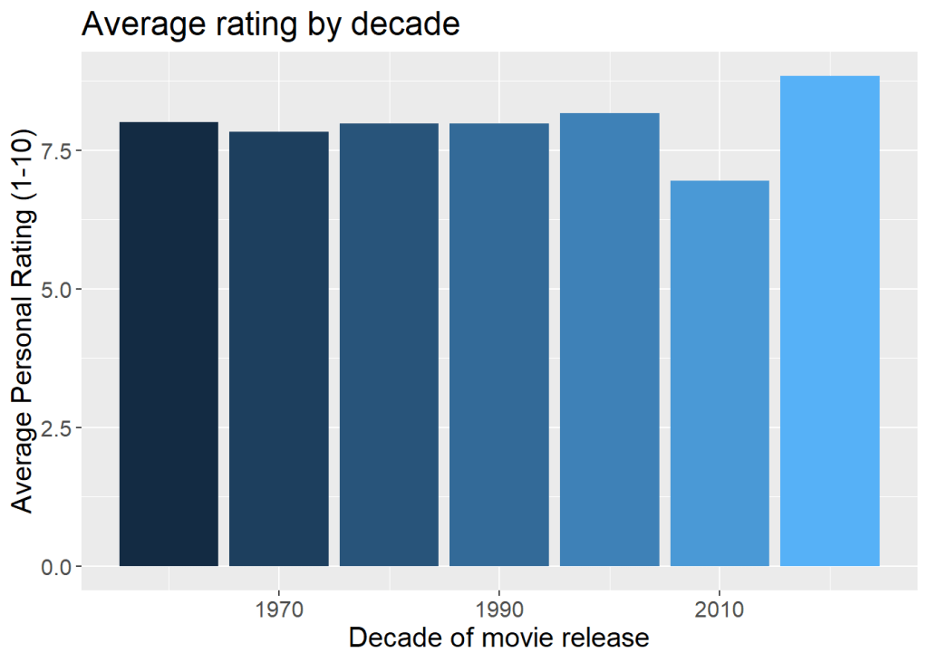
Visually, it looks like there is no obvious trend one way or the other. Since there are some decades with very few ratings and others with many, the visual differences may not mean much. To test this, I performed an analysis of variance (ANOVA) test to see if there was any statistical significance between each decade’s ratings. I found that there was no statistical significance (p = 0.125), though the p-value was rather low. Next year when I have more data to analyze, I will check this again and see if it holds true.
## ANOVA to test differences
summary(aov(personal_rating~decade, data = m))

##             Df Sum Sq Mean Sq F value Pr(>F)
## decade       1   7.18   7.184   2.409  0.125
## Residuals   73 217.71   2.982
I was also curious to see if I had a preferential difference for giving movies in certain genres higher ratings. As you can see below, it certainly looks like there might be a trend. For this plot, I removed genres that had fewer than three entries for legibility’s sake.
## Removing any genres with less than 3 entries (just for aesthetics sake)
small_gen = m %>%
  group_by(genre1) %>%
  filter(n() > 3)
## Creating a table of average scores and transforming it from largest to smallest
avgg = summaryBy(personal_rating~genre1, data = small_gen, FUN = mean, na.rm = TRUE)
avgg = transform(avgg, genre1 = reorder(genre1, -personal_rating.mean))
## Plotting with ggplot
gavgg = ggplot(data = avgg, aes(x=genre1, y = personal_rating.mean, fill = genre1))
gavgg + geom_col() + labs(title="Average rating by primary genre", x = "Genre", y = "Average Rating (1-10)") + theme(text = element_text(size=15), axis.text.x = element_text(angle = 90), legend.position = "none")
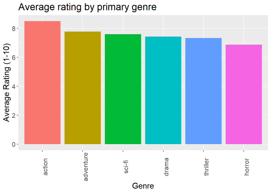
To test to see if there is in fact a preferential difference in how I rate movies based on genre, I ran another ANOVA (leaving in the genres with < 3 movies). Again I found that there was no statistical significance (p = 0.185). It’s nice to know that at least I don’t play favorites!
## Significant difference between scores?
summary(aov(personal_rating~genre1, data=m))

##             Df Sum Sq Mean Sq F value Pr(>F)
## genre1       9  37.62   4.180   1.451  0.185
## Residuals   65 187.27   2.881
Here is a plot of all the concepts discussed above combined.
g = ggplot(data = m, aes(x=year, y=personal_rating, color=genre1))
g + geom_point() +
labs(title="Personal Rating by Year of Movie Release", y = "Personal Rating (1-10)", x="Year of movie release", color = "Primary genre") + theme(text = element_text(size=15))

Right now, I am working on creating a linear model that I can use to predict my personal movie ratings based on the meta-data of the movie (year, budget, runtime, etc.). I have also expanded my sheet to include more meta-information as well as provide additional aspects of the movie to rate, rather than just my overall personal score. Next year, I should have much more robust data to analyze.
On to the 2020 Bobson Awards
Every movie lover knows the temptation of spamming friends and family with movie recommendations. Looking over all of the movies I watched this year, my natural response was to write down a list of some of my favorites to send to people. In an admittedly self-aggrandizing form, I decided to do this with flair and create the first annual Bobson Awards.
(Friends know that I often use the moniker “Al Bobson” online (Alexander shortened to “Al”, Robertson shortened to “Bobson”).)
Without further ado, the categories and nominations are below. I was originally going to limit myself to five nominations per category but they’re my stupid made-up awards so I get to make the rules (and I say there are no rules).
| Best Overall New (to me) Overall favorite new-to-me movie |
| Midsommar |
| Portrait of a Lady on Fire |
| The Thing (1982) |
| Knives Out |
| Crouching Tiger Hidden Dragon |
| The Farewell |
| John Wick |
| Best Rewatch Movies that I thought were even better the second time around |
| Knives Out |
| Spirited Away |
| Parasite |
| Midsommar |
| Cloud Atlas |
| Eye Candy Movies my eyes couldn’t get enough of |
| Ad Astra |
| Spirited Away |
| Midsommar |
| Annihilation |
| Mandy |
| Earworms Movies that got stuck in my head and I couldn’t stop thinking about |
| Portrait of a Lady on Fire |
| Do the Right Thing |
| Cloud Atlas |
| The Thing (1982) |
| There Will Be Blood |
| Midsommar |
| Ghost in the Shell (1995) |
| Spirited Away |
| Should have been an email Movies that drug on far too long |
| Ad Astra |
| Mandy |
| Susperia |
| The Head Hunter |
| Surprise! Movies that far exceeded my expectations |
| Ponyo |
| The Man Who Killed Hitler and then Killed the Bigfoot |
| Texas Chainsaw Massacre |
| Evil Dead 2 |
| John Wick |
In Closing
All in all, this was a fun project to test my chops with R and to revisit some of my favorite films of this year. If you have any tips for coding or recommendations for movies to watch in 2021, please let me know!

Leave a reply to Britt Cancel reply